Kinematics

Kinematics is the study of motion without the consideration of what causes that motion or collisions. We'll get to the topics of forces and collisions later. Kinematics is a fundamental part of any good simulation or physics engine. Even the simplest of games involve at least one object in motion across the screen. Take the game Pong, for example. The "ball" moves from one end of the screen to the other along a straight line, as the paddles move up and down in response to the players' controllers. This is about the simplest of games possible, and yet it is replete with challenges best solved through the application of Kinematics. In this chapter, we will look at the fundamental elements of motion, starting with a definition of our basic quantities and system of measure. After the introduction of our quantities, we'll see how these fundamental quantities can be used to create secondary quantities that describe motion and eventually arrive at four equations that will allow us to solve nearly any kinematics problem. The point of all this is, of course, to be able to model motion realistically in a game or simulation, so the final part of this chapter will introduce some algorithms that can be used to approximate the motion of an object. All algorithms have their advantages and disadvantages, and we'll discuss both.

Fundamental Quantities

When thinking about trying to describe the motion of an object, we quickly run into the issue of how to take measurements. We first need to understand what are the most fundamental quantities we can measure and which are derived quantities. As it happens, there are only three truly fundamental quantities, quantities that cannot be derived from combinations of other quantities. These three fundamental quantities are

• Length,
• Mass,
• and Time.

Combinations of these quantities produce all the other quantities that we can possibly measure. Now, we need a way to measure these fundamental quantities. There are many different measurement systems, but our focus will be on the Metric System.

The Metric System

The Metric System was conceived by French scientists in the late 1700s as a way to standardize and simplify units of measure. The intent was for there to be a single unit of measure for each of the three fundamental quantities that could be multiplied or divided by factors of 10 to provide larger or smaller secondary units. The current International System of Units, or Le Système International d'Unités (SI system), was formalized in 1960 and established the three base units as

• Meter (length)
• Kilogram (mass)
• Second (time)

This mks-system overrode the previous preference for centimeters, grams, and seconds, cgs-system.

The meter, kilogram, and second have also undergone significant revision in how they are defined. Originally, the meter was defined as one ten-thousandth of the distance along the line from the North Pole to the Equator that passes through Paris, France. Now the meter is defined as the distance a beam of light will travel in a vacuum after 1⁄299,792,458 seconds. This, obviously, relies on the definition of a second. Originally, the second was defined such that there were 86,400 seconds in one solar day. Now, the definition is much more precise. Here's the current definition from the Bureau International des Poids et Mesures:

The second is the duration of 9,192,631,770 periods of the radiation corresponding to the transition between the two hyperfine levels of the ground state of the Cs-133 atom.

The kilogram is perhaps the least precisely defined of the three fundamental units. The kilogram is still defined as the mass of the "international prototype of the kilogram". The international prototype is essentially a lump of iridium-platinum alloy metal kept at a precise temperature, pressure.

Unit Conversion

The simplicity of the metric system lies in the ability to describe very large or very small quantities using the same base-unit and a power-of-ten multiplier. Consider the difficulty in determining how many inches there are in a mile. The conversion factors that one has to use are 1760 yards to one mile, 3 feet to one yard, and 12 inches to one foot. In each case, simple "in your head" conversions are not practical unless you're a real arithmetic wiz! Determining how many centimeters in a kilometer is far more straight forward. The prefix, kilo- and centi-, refer to a power of ten. Kilo- means 1000, so one kilometer is equal to 1000 meters. Centi- means one hundredth, 0.01, so there are 100 centimeters to one meter, or one centimeter is 0.01 meters. When converting from one metric unit to another, the process involves either multiplying or dividing by a power of ten which can be done on one's head. Here is a list of commonly used unit prefixes:

Prefix	Symbol	Exponent	Multiplier
Tera	T	1012	1,000,000,000,000
Giga	G	109	1,000,000,000
Mega	M	106	1,000,000
kilo	k	103	1,000
centi	c	10-2	0.01
milli	m	10-2	0.001
micro	$\mu$	10-2	0.000001
nano	n	10-9	0.000000001

As nice as the metric system is, there will be times when one will need to work with and convert non-metric units. When converting from one unit to another, consider the process as always multiplying by one. Keep in mind that the purpose of a unit conversion is not to change the value of the quantity, only the units used to measure that value. For example, suppose we'd like to determine how many feet there are in 9 yards. Our conversion factor between yards and feet is 1 yd = 3 ft. Now we set up our conversion using this factor so that the unit we don't want is canceled out and we're left with the new unit we do want.

(1)

\begin{align} 9 yd \cdot \left( \frac {3 ft} {1 yd} \right) = \frac {9 \cdot 3 ft} {1} = 27 ft \end{align}

As a completely unrelated piece of trivia, the phrase "the whole nine yards" refers to the fact that the ammunition belts for most fighter aircraft during WWII were 27 feet long, so if you emptied your belt into a single target, you gave it "the whole nine yards."

Let's look at some other examples of unit conversions:

Example:
Convert 24 miles to meters:
1 mile = 1609 m
$24 ~mi \cdot \left( \frac {1609 ~m} {1 ~mi} \right) = 24 \cdot 1609 ~m = 38,616 ~m$

Exercise:
Convert 2.56 m to feet:
1 m = 3.28 ft

>> Solution <<

$2.56 ~m \cdot 3.28 \frac {ft} {m} = 8.40 ~ft$

When converting compound units, such as those for velocity, treat the problem as two back-to-back problems. In the following example of a velocity conversion, we'll convert the length units first and then the time units. Each step is no different than the process shown above, its just that we're performing two conversions one after the other.

Example:
Convert 300 km/hr to m/s:
1 km = 1000 m and 1 hr = 3600 s
$300 \frac {km} {hr} \cdot \frac {1000 ~m} {1 ~km} \cdot \frac {1 ~hr} {3600 ~s} = 83.3 \frac {m} {s}$

Exercise:
Convert 70 mph to m/s:
1 mi = 1609 m and 1 hr = 3600 s

>> Solution << 

$70 \frac {mi} {hr} \cdot \frac {1609 ~m} {1 ~mi} \cdot \frac {1 ~hr} {3600 ~s} = 31.3 \frac {m} {s}$

1D Motion

When trying to describe the motion of an object, we can begin by asking three simple question:

1. How far did the object move?
2. How fast was the object moving?
3. Was the object's speed getting faster or slower?

These three questions can be answered using the three basic quantities of motion: displacement, velocity, and acceleration. All three of these quantities are vector quantities, meaning that direction is important! In our first look at motion, we'll stick to a single dimention, but even in a 1D-case we need to treat the direction carefully. Before starting a problem, establish a coordinate system and indicate the origin and which direction is to be considered positive. Often in a game environment, this decision is made for you already. For example, typical 2D screen coordinates define the origin to be in the upper left corner with +x directed to the right and +y directed downward. In either case, be sure you have specified which direction is positive and where the origin is before you begin.

Displacement and Position

Displacement, distance, and position are related but not identical quantities. However, knowing each of these is important when describing the motion of an object. Let's consider first the quantity, position. Position is simply the location of the object relative to your defined coordinate system. For an everyday example, consider driving down an interstate. If you're driving on an even-numbered interstate, such as I-70, the milemarker posts mark your position along the interstate relative to the western state boundary. As you move east, your position increases in value, and as you move west, your position decreases in value. The value of displacement is the difference between your final and initial positions. This is different than the distance in a subtle way. Displacement not only states how far apart your final and initial positions are, but also the direction of your final position relative to your initial position.

Example:
Suppose you get on an interstate at Exit #118 and you stop at a truck stop at Exit #28. What are you initial and final positions, your distance travelled, and your displacement?

Your initial position is x_i = 118 mi, and your final position is x_f = 28 mi.
The distance you traveled is 90 mi, but the displacement is x_f-x_i= -90 mi, or 90 mi east.

Velocity

Velocity is a measure of how fast and in what direction your position changes. More formally, the velocity of an object is the time-rate-of-change in its position:

(2)

\begin{align} v = \frac {\Delta x} {\Delta t} \end{align}

If the velocity is to be found over a large interval of time, the above equation can be written as

(3)

\begin{align} v = \frac {x_f - x_i} {t} \end{align}

The units for velocity are units of distance per unit of time, so the standard metric unit is $m/s$. Other possible units include $mi/hr$, $ft/s$, and $pixels/step$. Here we must be careful and state that the velocity as calculated above is the average velocity over the time interval, $t$. Let's consider again our example of driving down the interstate. If we arrive at Exit #28 1.5 hours after we get on the interstate at Exit #118, then our average velocity for the trip is our change in position divided by the total elapsed time,

(4)

\begin{align} v = \frac {118 ~mi - 28 ~mi} {1.5 ~hr} = 60 ~mi/hr~. \end{align}

This does not necessarily mean that we were travelling 60 mph the entire trip. There may have been times when we were moving at 70 mph and other times when we had to slow down to 50 mph. We only know that our average speed for the entire trip was 60 mph. As we shrink the interval over which we measure the velocity, we can get closer and closer to the instantaneous velocity. The instantaneous velocity is what you read from your speedometer. Its the velocity of an object at a single moment in time.

Example:
A fastball travels the 62.5 ft from the pitcher's mound to home plate in 0.463 s. What is the speed of the ball in ft/sec? How about in mi/hr?

$v = \frac {62.5 ft} {0.463 s} = 135 ft/sec$
$v = 135 \frac {ft} {s} \cdot \frac {1 ~mi} {5280 ~ft} \cdot \frac {3600 ~s} {1 ~hr} = 92.0 ~mph$

Exercise:
A state trooper clocks a car as taking 5.4 s to travel between two posts on a highway 1/8th of a mile apart (0.125 mi). How fast is this car moving? Is he going to get a ticket if the speed limit is 70 mph?

>> Solution <<

$\Delta x = 0.125 ~mi$
$t = 5.4 ~s \cdot \frac {1 ~hr} {3600 ~s} = 0.0015 ~hr$
$v = \frac {\Delta x} {t} = \frac {0.125 ~mi} {0.0015 ~hr} = 83 ~mph$
Busted!

Acceleration

Acceleration is a measure of how quickly the velocity of an object changes. In common language, acceleration refers to an increase in speed whereas deceleration refers to a decrease in speed, but here we will use the term acceleration for both cases. A deceleration is simply an acceleration with a negative value. The formal definition for acceleration is the time rate of change in velocity:

(5)

\begin{align} a = \frac {\Delta v} {\Delta t} . \end{align}

If the acceleration is constant over a given interval of time, then the acceleration can be found precisely by

(6)

\begin{align} a = \frac {v_f - v_i} {t} \end{align}

The units for acceleration are units of velocity divided by units of time, so the standard metric unit is $\frac {m/s} {s} = m/s^2$. Other units include $ft/s^2$, $mph/s$, or $pixels/step^2$.

Example:
A sports car accelerates from rest to 60.0 mph in 3.9 s. What is its acceleration in $m/s^2$ ?
$v_i = 0$ ("from rest" means its initial velocity is zero.)
$v_f = 60 \frac {mi} {hr} \cdot \frac {1609 ~m} {1 ~mi} \cdot {1 ~hr} {3600 ~s} = 26.8 \frac {m} {s}$
$a = \frac {26.8 - 0} {3.9} = 6.9 \frac {m} {s^2}$

Exercise:
A boat starts from rest and accelerates at $1.68 \frac {m} {s^2}$. How fast is the boat travelling after 2.59 s?

>> Solution <<

$a = \frac {v_f - v_i} { t }$, but $v_i = 0$, so $a = \frac {v_f} {t}$
$a \cdot t = v_f$
$v_f = 1.68 \frac {m} {s^2} \cdot 2.59 ~s = 4.35 \frac {m} {s}$

Equations of Motion

Uniform Acceleration

If, over a given interval of time, the acceleration is constant, there are four equations of motion that can be derived from the definitions of the velocity and acceleration given above. Although the acceleration is constant over our time interval, the velocity is not. The final velocity over the interval can be found solving Eq 6

(7)

\begin{equation} v_f = v_i + a t \end{equation}

However, since the velocity will be changing at a constant rate, the average velocity, the initial velocity, and the final velocity share a simple relationship:

(8)

\begin{align} v_{avg} = \frac {v_i + v_f} {2} \end{align}

With this key relationship, we can begin to derive our equations of motion.

(9)

\begin{eqnarray} v_{avg} &=& \frac {\Delta x} {\Delta t} \\ &=& \frac {x_f - x_i} {t} \\ \frac {v_i + v_f} {2} &=& \frac {x_f - x_i} {t} \\ \end{eqnarray}

Solving for the final position yields

(10)

\begin{align} x_f = x_i + \left( \frac {v_i + v_f} {2} \right) t \end{align}

Combining
Substituting the expression for $v_f$ from Eqs. 7 into 10 allows us to determine final position given initial velocity, acceleration, and time.

(11)

\begin{eqnarray} x_f &=& x_i + \left( \frac {v_i +v_i + a t} {2} \right) t\\ &=& x_i \left( \frac {2 v_i + a t} {2} \right) t\\ &=& x_i \left(v_i + {\scriptstyle \frac{1}{2}} a t \right) t\\ \end{eqnarray}

Finally, we have

(12)

\begin{align} x_f = x_i + v_i t + {\scriptstyle \frac{1}{2}} a t^2 \end{align}

Solving Eq. 7 for time,

(13)

\begin{align} t = \frac {v_f - v_i} {a} , \end{align}

we can eliminate time from our equation by substituting our expression into Eq. 10.

(14)

\begin{eqnarray} x_f &=& x_i + \left( \frac {v_f + v_i} {2} \right) \cdot \left( \frac {v_f - v_i} {a} \right) \\ &=& x_i + \frac { \left( v_f + v_i \right) \cdot \left( v_f - v_i \right) } {2 a} \\ 2 a \left( x_f - x_i \right) &=& \left( v_f + v_i \right) \cdot \left( v_f - v_i \right) \\ v_f^2 - v_f v_i + v_f v_i - v_i^2 &=& 2 a \left( x_f - x_i \right) \\ v_f^2 - v_i^2 &=& 2 a \left( x_f - x_i \right) \\ \end{eqnarray}

Solving finally for $v_f^2$ reveals our fourth and last kinematic equation,

(15)

\begin{align} v_f^2 = v_i^2 + 2 a \left( x_f - x_i \right) \end{align}

Now we have four equations, Eqs 12, 10, 7, and 15, with which we can solve any given uniform acceleration problem.

The Four Kinematic Equations of Motion

(16)

\begin{eqnarray} x_f &=& x_i + v_i t + {\scriptstyle \frac{1}{2}} a t^2 \\ x_f &=& x_i + \left( \frac {v_i + v_f} {2} \right) t \\ v_f &=& v_i + a t \\ v_f^2 &=& v_i^2 + 2 a \left( x_f - x_i \right) \\ \end{eqnarray}

Example:
In a previous example, we saw that a sports car accelerated from rest to a speed of 60 mph (26.8 m/s) in 3.90 s. How much distance does the car cover during this time?

$v_i = 0$, $v_f = 26.8 ~m/s$, $t = 3.90 ~s$, and $x_i = 0$. $x_f = ?$
Use Eq. 10 since it has velocities, distances, and time which we know, and doesn't contain acceleration which we don't know.
$x_f = x_i + \left( \frac {v_i + v_f} {2} \right) t$
Eliminate zero-valued quantities. This will help make the algebra we need to do easier.
$x_f = \left( \frac {v_f} {2} \right) t$
Now we can plug in our known values and evaluate $x_f$.
$x_f = \frac {26.8} {2} \cdot 3.90$
$x_f = 52.3 m$

Exercise:
A train moving at 35 m/s tries to stop in a hurry. It finally comes to a stop after traveling 3/4 of a mile (1207 m). What is the train's acceleration and how long does it take for the train to stop?

>> Solution <<

$v_i = 35 \frac {m} {s}$, $v_f = 0$, $x_i = 0$, $x_f = 1207 ~m$
Find the acceleration using Eq. 15
$v_f^2 = v_i^2 + 2 a \left( x_f - x_i \right)$
Eliminate zero-valued quantities.
$0 = v_i^2 + 2 a x_f$
Solve for $a$
$a = - \frac {v_i^2} {2 x_f}$
$a = - \frac {35^2} {2 \cdot 1207} = -0.507 \frac {m} {s^2}$

Find the time using Eq. 10
$x_f = x_i + \left( \frac {v_i + v_f} {2} \right) t$
$x_f = \frac {v_i} {2} t$
$t = \frac {2 x_f} {v_i}$
$t = \frac {2 \cdot 1207} {35} = 69.0 ~s$ (over a minute!)

Free Fall Motion

Galileo demonstrated in his experiments that a falling body will be accelerated at a constant rate regardless of its mass. Supposedly, he demonstrated this most dramatically by dropping various weight stones off of the Leaning Tower of Pisa. That may or may not be true, actually, but it makes for a good story. Regardless of whether he performed this very public act of science or not, the fact remains that all things, regardless of mass, are accelerated by gravity at the same rate. This is contrary to what Aristotle believed who stated that heavier object must fall faster. Its easy to see how Aristotle may have thought this. If you drop a feather and a hammer at the same time, the hammer obviously will fall faster, but there's a complication. Air resistance affects the motion of the feather far more than the motion of the hammer. If you dropped a feather and a hammer somewhere where there was no air to get in the way, say the Moon for example, then the two objects would indeed fall at the same rate. This fact was verified by Commander David Scott during the Apollo 15 mission.

When we consider objects of sufficient mass that we can neglect air resistance, they are all accelerated by gravity at the same rate, so we give this acceleration its own symbol, $g$ such that(17)

\begin{align} g = 9.8 {\scriptstyle \frac {m} {s^2}} \end{align}

When we consider the four kinematic equations, Eqs. 12, 10, 7, and 15, as they apply to objects in free-fall, we can make some simple substitutions and arrive at four equations that describe falling bodies. Since when considering falling bodies, objects will be moving in the vertical direction, we'll substitute $y$ for $x$. If we assume that upwards is the positive direction, then the acceleration, $a$ can be substituted with $-g$. Doing so gives us the following equations:

(18)

\begin{align} y_f = y_i + v_i t - {\scriptstyle \frac{1}{2}} g t^2 \end{align}

(19)

\begin{align} y_f = y_i + \left( \frac {v_i + v_f} {2} \right) t \end{align}

(20)

\begin{equation} v_f = v_i - g t \end{equation}

(21)

\begin{align} v_f^2 = v_i^2 - 2 g \left( y_f - y_i \right) \end{align}

Example:
A tennis player tosses the ball up from an initial height of 1.5 m with a speed of 5.2 m/s. What is the maximum height the ball reaches?

$v_i = +5.2 ~m/s$, $y_i = 1.5 ~m$, $v_f = 0$. At the top of a objects arc, its vertical velocity will always be zero.
Use Eq 26 to find $y_f$
$v_f^2 = v_i^2 - 2 g \left( y_f - y_i \right)$
Eliminate zero-valued quantities.
$0 = v_i^2 - 2 g \left( y_f - y_i \right)$
Solve for $y_f$.
$y_f = y_i + \frac {v_i^2} { 2 g}$
$y_f = 1.5 + \frac {5.2^2} {2 \cdot 9.8} = 2.9 ~m$

Example:
A ball is thrown upward at 10.3 m/s from the top edge of a 25-m high building. How long will it take for the ball to reach the ground below?
$v_i = 10.3 ~m/s$, $y_i = 25 ~m$, $y_f = 0$ Its tempting to say that $v_f =0$, but realize that the ball will be moving quite fast when it strikes the pavement below. It will only come to a rest after it hits the ground.
Use Eq. 23 to find the time.
$y_f = y_i + v_i t - {\scriptstyle \frac{1}{2}} g t^2$
This equation is quadratic, so we'll need to use the Quadratic Formula, but first we need to get the above equation into standard form, $a x^2 + b x + c =0$.
${\scriptstyle \frac{1}{2}} g t^2 - v_i t + (y_f - y_i) = 0$
$a = {\scriptstyle \frac{1}{2}} g = 4.9$
$b = - v_i = -10.3$
$c = y_f - y_i = -25$
Therefore,
$t = \frac { -b \pm \sqrt {b^2 - 4 a c} } {2 a}$
This gives us two possible answers, one of which is physical and the other of which is not.
$t_- = -1.44 ~s$ This is clearly not possible.
$t_+ = 3.54 ~s$ This is our answer.

Projectile Motion

One of the convenient aspects of displacement, velocity, and acceleration all being vector quantities, is that each of the three components for the x-, y-, and z-directions are all independent of one another. In other words, an acceleration in the z-direction will only affect the velocity in the y-direction. The x and y-components of the velocity remain unchanged. This permits us to look at a projectile in flight as three separate kinematic problems, rather than trying to tackle the whole problem at once.

If we consider a projectile in flight and ignore the complication of wind resistance, we can see that it will always be a 2D problem. The x-axis we orient along the projectile's horizontal path, and the y-axis in the vertical direction. For this case, the acceleration in the horizontal direction is zero, $a_x=0$, and in the vertical direction is the acceleration due to gravity, $a_y=-g$. Applying these conditions to the kinematic equations we derived in previously in Kinematics, we can create five equations that describe the motion of any projectile.

Horizontal Motion:

(22)

\begin{equation} x_f = x_i + v t \end{equation}

Vertical Motion:

(23)

\begin{align} y_f = y_i + v_i t - {\scriptstyle \frac{1}{2}} g t^2 \end{align}

(24)

\begin{align} y_f = y_i + \left( \frac {v_i + v_f} {2} \right) t \end{align}

(25)

\begin{equation} v_f = v_i - g t \end{equation}

(26)

\begin{align} v_f^2 = v_i^2 - 2 g \left( y_f - y_i \right) \end{align}

When using these five equations, it will be quite common to solve one direction for time in order to gain information about the motion in the other direction. Consider this example:

Example:
A stunt car runs off of a 15-m high building at a speed of 22 m/s. How far away from the building does the car land?

Since the initial height of the car is know, the time it takes to fall can be calculated. Keep in mind that its horizontal speed is irrelevant to the time it takes to fall, only the vertical velocity, which is zero here, matters.

$v_{y,i} = 0$
$y_i = 15 m$
$y_f = 0$
Looking at Eq. 23, $0 = y_i - {\scriptstyle \frac{1}{2}} g t^2$
Solving for t, $t = \sqrt { \frac {2 * y_i} {g} } = 1.75 s$
Inserting time into Eq. 22, $x_f = x_i + v_x t = 22 \frac {m} {s} 1.75 s = 38.5 m$

Very often, the initial velocity is given as a vector in magnitude and direction form rather than as separate horizontal and vertical components as in the above problem. In this case, one must first resolve the vector into the horizontal and vertical components before beginning the problem. If the direction for the velocity is given as an angle above the horizontal, then the initial x- and y- components are given by

(27)

\begin{align} v_x = v_i \cos \left( \theta \right) \end{align}

(28)

\begin{align} v_{yi} = v_i \sin \left( \theta \right) \end{align}

Exercise:
A shotput leaves the thrower's hand at a height of 2.20 m and with a velocity of 10.6 m/s at 40 degrees above the horizontal. How far away from the thrower does the shotput land?

>> Solution <<

$y_i = 2.20, y_f = 0, x_i = 0,$,
$v_x = 10.6 \cos \left( 40 \right) = 8.12 m/s$,
$v_+{yi} = 10.6 \sin \left( 40 \right) = 6.81 m/s$
We can find the horizontal distance with $x_f = x_i + v_x t$, but we need $t$ first.
Looking at the motion in the y-direction, we can get the time from the following:
$y_f = y_i + v_{yi} t - {\scriptstyle \frac{1}{2}} g t^2$
Zeroing out the terms we don't need still leaves us with a quadratic equation,
$0 = 2.20 + 6.81 t - 4.9 t^2$ where,
$a = -4.9$
$b = 6.81$
$c = 2.20$
Applying the quadratic formula and solving for t yields
$t = \frac { -b \pm \sqrt {b^2 - 4 a c} } {2 a}$
$t = 1.66 s$
Plugging this time back into our equation for the horizontal position, we can get the total range.
$x_f = 8.12 * 1.66 = 13.5 m$

If the projectile is fired over flat, level ground, then we can derive a simple equation that will yield the total range of the projectile, so long as we ignore air resistance. If we start with $x_i = 0$, then Eq. 22 reduces to $x_f = v_x t$. If the initial velocity is known, then all that's needed to find the total distance, $x_f$, isthe total time, $t$. To find the total time, we focus on the fact that if the projectile takes off and lands at the same height, then $y_f = y_i$ so that Eq. 23 becomes,

(29)

\begin{align} 0 = v_{yi} t - {\scriptstyle \frac{1}{2}} g t^2 \end{align}

We can divide both sides by $t$ since we know $t \neq 0$ and then solve.

(30)

\begin{align} t = \frac {2 v_{yi}} {g} \end{align}

Inserting this into our equation for the total range and making the substitutions of $v_x$ and $v_{yi}$ given in Eqs. 27 and 28 gives us our final solution.

(31)

\begin{align} x_f = v_i \cos \left( \theta \right) \cdot \frac {2 v_i \sin \left( \theta \right)} {g} x_f = \frac {{v_i}^2} {g} 2 \cos \left( \theta \right) \sin \left( \theta \right) \end{align}

Recalling that $2 \cos \left( \theta \right) \sin \left( \theta \right) = \sin \left( 2 \theta \right)$

(32)

\begin{align} x_f = \frac {{v_i}^2} {g} \sin \left( 2 \theta \right) \end{align}

If we examine Eq. 32 closely, we can see that for a given initial velocity, there is one angle that yields a maximum range, 45 degrees. Lets look at an example:

Example
A soccer player kicks a ball with an initial speed of 25.9 m/s at an angle of 35 degrees. How far away from the player does the ball land?
$v_i = 25.9 m/s, \theta = 35$
$x_f = \frac {{25.9}^2} {9.8} \sin \left( 2 \cdot 35 \right)$
$x_f = 64.3 m$

That was straightforward, plug in the numbers and crunch out the result. Let's look at a different problems.

Exercise
The distance from home plate to the center field fence at Kauffman Stadium (Royals Stadium) is 405 ft. If a baseball leaves a batter's bat at a speed of 120 mph, at what minimum angle must the ball leave if its to be a home run and clear the center field fence?

>> Solution <<

The first step is to get all of the data into a consistent set of units. Let's convert everything into standard metric units.
$405 ft \cdot \frac {1 m} {3.281 ft} = 123.4 m$
$v_i = 120 mph \cdot \frac {1609 m} {1 mile} \cdot \frac {1 hour} {3600 s} = 53.6 m/s$
Now lets solve for the angle, $\theta$.
$x_f = \frac {{v_i}^2} {g} \sin \left( 2 \theta \right)$
$\frac {g x_f} {{v_i}^2} = \sin \left( 2 \theta \right)$
$\theta = \frac {1} {2} \sin^{-1} \left( \frac {g x_f} {{v_i}^2} \right)$
$\theta = 0.5 \sin^{-1} \left( \frac {9.8 \cdot 123.4} {{53.6}^2} \right)$
$\theta = 12.4 deg$

Integration Methods

If the acceleration is constant, then one can easily use the four kinematic equations. However, the acceleration for most objects, either real or in-game, is seldom constant. Therefore, we'll need a different method for solving for the motion of these objects moving with a non-uniform acceleration. The key point to our evaluations will be to consider the small changes from one time-step in our game or simulation to another.

Forward Euler Method

Although over large time intervals, the acceleration changes, we can make the assumption that acceleration is constant over a very small interval $\Delta t$. Let's re-examine our definition of acceleration from Eq. 5. If we multiply both sides of Eq. 5 by $\Delta t$, we get

(33)

\begin{align} \Delta v = a \Delta t \end{align}

Here, $\Delta v$ is the difference in velocity from the previous time-step to the current time-step. So we can rewrite the above equation as something that resembles Eq. 7, except instead of some large value of time, we use a the small difference in time between the previous and current time-steps.

(34)

\begin{align} v_i = v_{i-1} + a_{i-1} \Delta t \end{align}

A similar method can be used using Eq. 2 to find the current position for an object.

(35)

\begin{align} x_i = x_{i-1} + v_{i-1} \Delta t \end{align}

Here's a sample of code demonstrating the implementation of this method that models a projectile shot upwards at 49 m/s.

float dt = 0.1f;    //Set the time-step size in s.
float t = 0.0f;    //Set initial time to 0 s.
float y = 0.0f;    //Set initial position to 0 m.
float v = 49.0f;    //Set initial velocity to +49 m/s.
float a = -9.8f;    //Set acceleration to -g (-9.8 m/s^2).
while (y >= 0.0f ) {
    y += v * dt;    //Find the new position.
    v += a * dt;    //Find the new velocity.
    ///* If the acceleration is variable, this is where the new acceleration should be evaluated. */
    t += dt;        //Increment the time.
}
cout<<"The projectile flew for "<<t<<" s."

This method of moving an object forward in time is easy to code, and executes very quickly, however there are drawbacks. Our assumption here for Eq. 34 is that the acceleration is constant over $\Delta t$, and that the velocity is constant over $\Delta t$ for Eq. 35. These assumptions are obviously not correct, but if $\Delta t$ is small enough, the assumption is close enough to correct to yield decent results. As the size of $\Delta t$ increases, errors in this method become more and more apparent.

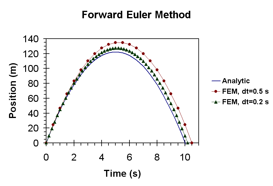
Notice in the picture above that the modeled motion approaches the analytic solution with smaller time-steps, but that in all cases, the object moves farther than it really should every time-step. This is equivalent to a gain in energy. In any simulation using Forward Euler, projectiles will fly farther than they should, and oscillations will grow over time. The video below is a good example of a bouncing ball modeled using Forward Euler and the effects of increasing energy.

Reverse Euler Method

The Reverse Euler Method (REM) differs from the Forward Euler Method (FEM) in that it uses the new value for velocity to calculate the new position rather than the old value. So the only change in Eqs. 34 and 35 is the subscripts.

(36)

\begin{align} v_i = v_{i-1} + a_i \Delta t \end{align}

(37)

\begin{align} x_i = x_{i-1} + v_i \Delta t \end{align}

This change in which velocity and acceleration one uses to calculate the new position and velocity necessitate a slight change in the implementation. Take careful note of the order of execution in the segment of code shown below as compared to the code shown for the FEM.

float dt = 0.1f;    //Set the time-step size in s.
float t = 0.0f;    //Set initial time to 0 s.
float y = 0.0f;    //Set initial position to 0 m.
float v = 49.0f;    //Set initial velocity to +49 m/s.
float a = -9.8f;    //Set acceleration to -g (-9.8 m/s^2).
while (y >= 0.0f ) {
    ///* If the acceleration is variable, this is where the new acceleration should be evaluated. */
    v += a * dt;    //Find the new velocity.
    y += v * dt;    //Find the new position.
    t += dt;        //Increment the time.
}
cout<<"The projectile flew for "<<t<<" s."

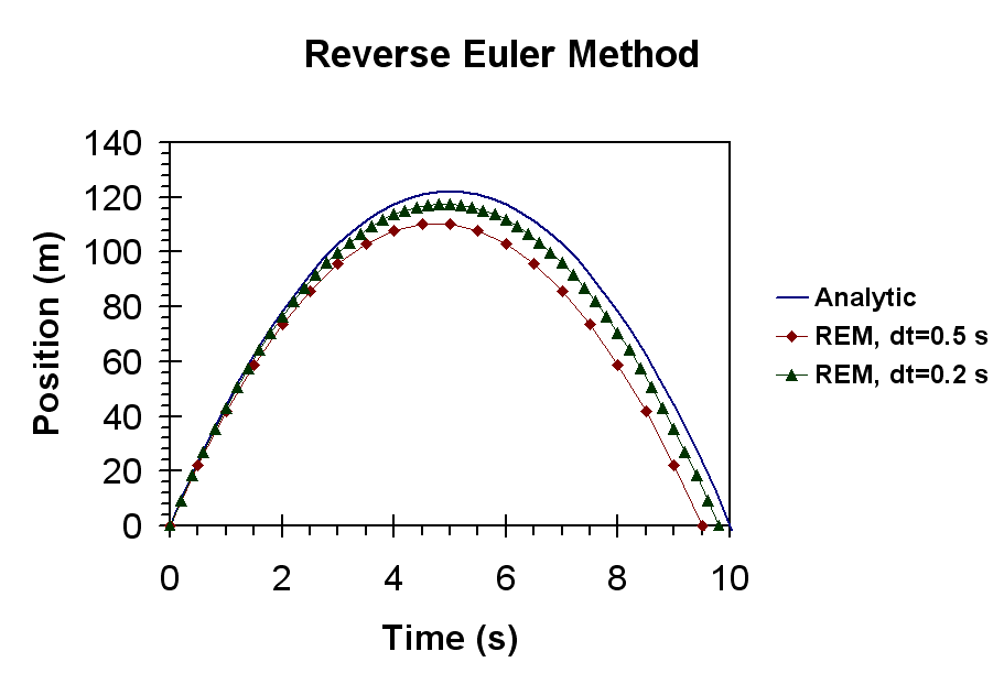
Whereas the Forward Euler Method adds energy over time to an object, the Reverse Euler Method removes it. Below is a simulation of the same particle thrown upward shown in the Forward Euler Method using REM. Notice that the modeled motion now falls short of the analytic solution.

Velocity Verlet

A more accurate method than Euler integration, but also more expensive, is Velocity Verlet. While verlet integration doesn't perfectly conserve energy in all circumstances, it matches the analytic solution exactly for uniformly accelerated systems such as projectile motion. In other energetically conservative systems such as spring oscillators, or motion under the influence of gravitation, the energy modeled by the velocity verlet algorithm oscillates around the analytic value. While this variation may be undesirable for a strictly precise physical simulation, for the purposes of most game physics engines, it is close enough to the actual physical behavior to produce realistic results over the time scales typical to most gameplay situations.

The essence of the velocity verlet method is to utilize the previous values of the position, velocity, and acceleration to calculate the new position via Equation Eq. (12). Before calculating the new velocity, however, one must next calculate the acceleration at the newly calculated position while retaining the value of the previous acceleration. This will require keeping two variables for the acceleration, one for the value from the previous frame and one for the value in the new frame. The new velocity is calculated via a modified version of Eq. (7) utilizing the average of the old and new accelerations. The full process flows as follows:

• Calculate the new position, $x_{i} = x_{i-1} + v_{i-1} * \Delta t + 0.5 * a * {\Delta t}^2$.
• Calculate $a_{i}$ using the new position, $x_{i}$, and the previous velocity, $v_{i-1}$.
• Use $a_{i}$ and $a_{i-1}$ to calculate the new velocity, $v_{i} = v_{i-1} + 0.5 * (a_{i} + a_{i-1}) * \Delta t$

This method precisely models uniformly accelerated motion, and does a good job at modeling velocity-dependent forces such as fluid resistance. Below is an example modelling a ballistic projectile while taking wind resistance into account.

float dt = 0.1f;    //Set the time-step size in s.
float t = 0.0f;    //Set initial time to 0 s.
float y = 0.0f;    //Set initial position to 0 m.
float v = 49.0f;    //Set initial velocity to +49 m/s.
float a = -9.8f;    //Set acceleration to -g (-9.8 m/s^2).
float anew = -9.8f; //Set the new acceleration to -g (-9.8 m/s^s)
float cwind = 0.2f;  //Set the coefficient of wind resistance to 0.2 kg/s.
while (y >= 0.0f ) {
    y += v * dt + 0.5f * a * dt * dt;    //Find the new position.
    anew = -9.8 - cwind * v;    //Find the new acceleration.
    v += 0.5f * (a + anew) * dt;    //Find the new velocity using the average of the old and new accelerations.
    a = anew;     //update the main acceleration variable with the new value.
    t += dt;        //Increment the time.
}
cout<<"The projectile flew for "<<t<<" s."

Note that we multiply by 0.5 rather than dividing by 2. Floating-point division is significantly more expensive than multiplication, so when possible, we choose to use multiplication. We also avoid the use of the CMATH intrinsic function pow() to simply square the value dt. The pow() function is useful when you need to raise a value to a arbitrary or fractional value, but it is extremely expensive computationally. It is significantly more efficient to simply execute dt * dt than to evaluate pow(dt, 2).

*Runga-Kutta

The Runga-Kutta method is a far more precise method of modeling motion, but the major drawback is the additional computations that are needed. For small programs and today's processors, this is typically not a problem, but as both the speed required from the simulation and the number objects to be simulated increases, the additional calculations will become problematic. The Runga-Kutta method also requires more memory in that one needs to keep track of at least five instead of only three variables for each object. The Runga-Kutta method can be extended to as many orders as the programmer desires, but for here, we will consider the Fourth Order Runga-Kutta method. This method is so widely used that its often referred to simply as the Runga-Kutta method, or as we'll refer to it here, RK4. Later, we'll look at this method with an acceleration that varies with both time and position, but for now, let us consider only time-varying values. In the FEM and REM, the previous values of acceleration, velocity, and position are destroyed as the new values are computed, but for the RK4 method, both the new and the previous values must be used.

(38)

\begin{align} x_i = x_{i-1} + \left( k_1 + 2 k_2 + 2 k_3 + k_4 \right) \frac {dt} {6} \end{align}

where $k_1$, $k_2$, $k_3$, and $k_4$ are given by

(39)

\begin{eqnarray} k_1 &=& v(x_{i-1}, t_{i-1}) = v_{i-1}\\ k_2 &=& v(x_{i-1}+k_1 \frac {dt} {2}, t_{i-1} + \frac {dt} {2}) \\ k_3 &=& v(x_{i-1}+k_2 {\scriptstyle \frac {dt} {2}}, t_{i-1} + \frac {dt} {2})\\ k_4 &=& v(x_{i}, t_{i}) = v_i \\ \end{eqnarray}

A similar scheme can be used for calculating the velocity. If the acceleration is constant, then the above scheme becomes much simplified:

(40)

\begin{align} x_i = x_{i-1} + \left( v_i + v_{i-1} \right) \frac {dt} {2} \end{align}

For a constant acceleration, the implementation of RK4 is quite straightforward, but it will require more variable declarations as shown in the code sample below.

float dt = 0.1f;        //Set the time-step size.
float t = 0.0f;        //Set initial time to 0 s.
float y = 0.0f;        //Set initial position to 0 m.
float ynew = 0.0f ;    //Initialize the new position variable.
float v = 49.0f;        //Set initial velocity to +49 m/s.
float vnew = 49.0f;    //Initialize the new velocity variable.
float a = -9.8f;        //Set acceleration to -g (-9.8 m/s^2).
while (y >= 0.0f ) {
    ///* If the acceleration is variable, this is where the new acceleration should be evaluated. */
    vnew = v + a * dt;                    //Find the new velocity.
    ynew = y + 0.5 * (v + vnew) * dt;        //Find the new position.
    t += dt;                            //Increment the time.
    v = vnew;        //Update the velocity variable
    y = ynew;        //Update the position variable
}
cout<<"The projectile flew for "<<t<<" s."

The biggest advantage of the RK4 scheme is that it more closely models the analytic solution than either FEM or REM, and therefore, larger time-steps can be used. Notice the far more precise agreement between the modeled positions in the graph shown below.

Questions and Exercises:

Conceptual Questions:

1. Why are the quantities of length, mass, and time considered "fundamental" quantities?
2. How are average and instantaneous velocities different?
3. The victor of the Indianapolis 500-Mile Race completes 200 laps around the 2.5-mile Indianapolis Motor Speedway. What is the total distance covered by the race winner? What is the total displacement?
4. Can an object have a zero velocity yet still have a non-zero acceleration? Defend your answer.
5. Identify the following quantities as either a displacement, a velocity, or an acceleration based upon the units used:
   • 150 m
   • 25 km/s
   • 49 px
   • 256 px/step
   • 13.7 mph/s
6. What are the advantages of using the Forward Euler Method as compared to higher-order integration methods? What are the disadvantages?
7. Explain the advantages and disadvantages to choosing a large time-step when using the Forward Euler method for modeling motion.

Problems:

1. How many centimeters are there in 0.476 km?
2. Convert the speed of 100.0 km/hr to units of m/s.
3. Given the following graph of acceleration vs. time, draw a velocity vs. time graph where the initial velocity is zero.
4. How long will it take an aircraft traveling at 368 m/s to travel from Kansas City to a St. Louis airport 223 miles away?
5. The Focus ZX3 SES can accelerate from 0-60 miles/hr in 10.3 seconds. What is the acceleration for the car in m/s²?
6. How much distance is covered by the Focus while accelerating from 0-60 miles/hour in 10.3 seconds?
7. A high-end sports car with good tires can accelerate 11 m/s². How long will it take the car to travel ¼ of a mile assuming the acceleration is constant?
8. What is the final velocity of the car from the previous question?
9. How fast must you throw a ball in order for it to reach a height of 23.1 m, the height of the Regnier Center? Assume the ball is released from an initial height of 2.1 m.
10. A car drives off the edge of a 42-m high cliff at a speed of 33 m/s. How long will it take for the car to reach the bottom?
11. How far from the face of the cliff will the car be when it eventually lands?
12. What is the final velocity (speed and direction) for the car when it eventually lands?
13. A baseball is thrown with a velocity of 23 m/s at an angle of 30 degrees. If the ball is launched from an initial height of 1.5 m, how long will it be in the air?
14. How far away will the ball travel before reaching the ground?
15. Complete the following tables for the position and velocity for a particle given the accelerations and a ∆t of 1.0 seconds.

Time (s)	Acceleration (m/s2)	Velocity (m/s)	Position (m)
0.0	1.0	0.0	0.0
1.0	2.0
2.0	5.0
3.0	10.0
4.0	9.0
5.0	8.0

16. Now compare your answers above to the actual, analytic values shown below. Why do they not agree with each other? What can be done to make the answers from the previous question come into better agreement with the real values?

Time (s)	Velocity (m/s)	Position (m)
0.0	0.0	0.0
1.0	1.3	0.6
2.0	4.7	3.3
3.0	12.0	11.3
4.0	24.5	29.6
5.0	36.0	59.9

You can find a full set of kinematic practice problems on Canvas, http://canvas.jccc.edu/.